

Introduction:
The contents of this section are primarily aimed at the basics of CIE colorimetry, color appearance, and concepts that are used in color management and digital image processing. It is neither a comprehensive overview of the Colorimetry nor an overview of color vision theory. For more detailed treatment of the topics, please see the Reference section at the end.
CIE Tristimulus and Chromaticity Coordinates:
Our visual system detects light using the light-sensitive organs that transmit generated impulses to the brain. The incident light is focused by cornea and the eye's lens to form an image being projected onto the retina. The retina is a light-sensitive layer at the back of the eye. The nerve cells in the retina that respond to light stimuli are called photoreceptors. These are classified into two types based on their shape: rods and cones. The area of the retina around the optical axis is designed for high resolution perception with a high concentration of cones. At the central point, each cone is connected by one optic nerve fiber to one point on the cortex of the brain. The cones are responsible for color vision. Observers with normal color vision have three different types of cones, commonly called S, M, and L. These abbreviated forms correspond to short, medium, and long wavelengths that each particular type of cones is sensitive to. Spectral sensitivities of the cones peak at 420 nm, 530 nm, and 560 nm, respectively. Rod receptors are more sensitive to light, but a large number of them are connected together before the sum of signals is sent to the brain. Thus they are good for sensing brightness and movement. In normal human observers, the spectral sensitivities of the three types of cones are linearly independent. The cones, as do any light detectors, integrate the light incident on them. This process reduces the entire spectrum of incident light to three signals, one for each type of cone, resulting in what is called trichromacy. The importance of trichromacy for the color imaging is that we can simulate almost any color by using just three primary colors - red, green, and blue.
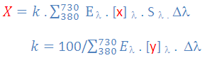
The trichromatic nature of human vision has been mathematically formulated by CIE (The Commission Internationale de l'Éclairage) to provide tristimulus values X, Y, and Z. CIEXYZ tristimulus values are thus fundamental measure of color. For the average human observer, under the same illuminant, stimuli with the same CIEXYZ coordinates are perceptually identical, meaning that the same color is perceived by an observer. This also means that the same color perceived under the same illuminant (and the same standard observer) has the same tristimulus values. From the measured color samples one would see that X, Y, and Z values approximately correspond to the red, green, and blue colors, respectively. In order to calculate tristimulus values, object spectra, spectral power distribution (SPD) of the illuminant, and the color matching functions ![]() are multiplied and summed over a range of wavelengths (usually from 380 nm to 730 nm in 10 nm intervals).
are multiplied and summed over a range of wavelengths (usually from 380 nm to 730 nm in 10 nm intervals).
 (I)
(I)Equation (I) shows how the X-tristimulus component of the CIEXYZ triplet is obtained. Y and Z components are calculated similarly using the corresponding color-matching functions [y] and [z]. S(λ) denotes the object spectrum (as reflectance, transmittance, or radiance), [x] is the color-matching function for the CIE 1931 or 1964 standard observer (tabulated), E(λ) is the relative spectral power distribution of a reference illuminant (also tabulated), and k is a normalizing constant. The original definition of the tristimulus values involved integration over the visible range of spectrum (I). However, as the analytical expressions for the color-matching functions do not exist, integration was replaced by summation over the wavelength intervals. For light sources and displays, S(λ) is given in quantities such as spectral radiance. If S(λ) is given in absolute units and k = 683 lm/W is chosen, Y yields an absolute photometric quantity called luminance. The only measurement data needed to calculate CIE tristimulus is the spectral power density (SPD) of the emission source (monitor) or reflectance spectra from a reflective object (e.g., print). In case of reflectance, measurements have to be done under a defined reference illuminant (frequently D50 - see the next section for more details). Processing of emission or reflectance spectra in a form of SPD requires some reference "white", e.g., spectrum of a white patch on your monitor, the ambient light, or the white ceramic target that is measured during spectrophotometer calibration. For the emission data, an equi-energy "Illuminant E" is chosen (spectral power density is equal to 1 at any wavelength). Strictly speaking, there is no reference illuminant E for the emissive case as the source (display) provides the light energy itself. For more details on the emission spectra -> XYZ calculations (r2XYZ), the following Excel spreadsheet is available as a reference (download here). Processing of up to 153 spectral data with the subsequent Bradford transformation and LAB calculation is implemented in the VBA macro mode. Another Excel spreadsheet is available from the Bruce Lindbloom's web site (see Spectral Calculator Spreadsheet). Calculations of the CIE tristimulus values for reflective materials are thoroughly described by Pascale and Sharma. Good news is that almost any spectrophotometer or colorimeter with a decent software will provide the XYZ values at the output.
Color-matching functions: also referred to as the CIE Standard Observer are intended to represent an average color vision of the normal human observer. Using three primary colors (R,G,B), the CIE performed experiments resulting in tables of values determining how much of each of the primaries is needed to match colors of a reference spectrum. The corresponding graphical results are called the color-matching functions (CMF). The interpretation of these graphs is that they show how much of each primary (called the tristimulus value) is needed to match unit of intensity of a single wavelength of light. Following example shows how color-matching functions are used in practice. Let's calculate tristimulus values for a monochromatic laser light at 694 nm. We will use the equation (I) described above. The corresponding color-matching functions (CIE 1931 2deg) at 694 nm are 0.016987, 0.006138, and 0.000000, respectively. Calculated tristimulus values XYZ are then: 276.7, 100.0, 0.0. The way we arrived to these numbers is following: each value of the color-matching functions at 694 nm was multiplied by 1 (S694), then again by 1 (E) for the illuminant E (hypothetical equal-energy spectrum), and then again by 1 for Δλ. Resulting values were normalized for the Y-component (division by 0.006138 and multiplication by 100). The corresponding (x,y) chromaticity values are x = 0.735 and y = 0.265 (calculated from eq. (II) discussed later). This would be the "purest", most saturated red that most people could see. Although the responsivity at 700 nm is already very low, even the light from some near-infrared laser diodes at wavelengths beyond 750 nm can be seen if that light is sufficiently intense. A wavelenght of about 760 nm is considered the red limit of the naked eye.
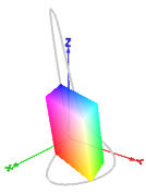
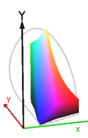
click here fancybox CMF testThe CIEXYZ system can be thought of as a 3-dimensional color space with orthogonal axes (Fig. 1). Corners of the green triangle in Fig. 1 have coordinates of XYZ primaries ([1,0,0], [0,1,0], [1,0,0]) and lie in the plane defined as X + Y + Z = 1. The CIEXYZ primaries are defined arbitrarily and are clearly outside the gamut of all real colors. As such, they are invisible. No color of light or surface can reproduce them as they are not physically realizable. However, this is of no consequence, because the system is computational rather than visual. XYZ mixing triangle completely contains the chromaticity space of all real, visible colors, so all colors can be described as the positive mixture of the XYZ imaginary lights. Another feature of the CIE XYZ primaries is that equal values of X, Y, and Z produce white. When tristimulus values of visible colors (i.e. the color matching functions) are projected onto the green unit plane, trace of the horseshoe shape becomes apparent (in blue). This so called "horseshoe" diagram is essentially a projection of 3-D XYZ values onto 2-D xy plane.
Figure 1: CIEXYZ to xy transformation
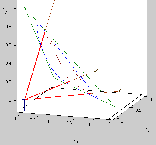
Contour of such projection represents boundary of the human gamut (colors that we can see). Red lines in Fig. 1 intersect the unit plane at primaries of any arbitrary gamut within the full gamut of all visible colors. Unfortunately, CIEXYZ values do not give any obvious representation of color and thus some other representations of tristimulus system are needed. One such system is the CIE 1931 xy-chromaticity diagram. The chromaticity coordinates x, y, and z are obtained by taking the ratios of the tristimulus values to their sum.
x = X/(X + Y + Z)
y = Y/(X + Y + Z)(II)
z = Z/(X + Y + Z)
and thus X = x/y . Y, Z = z/y . Y and x + y + z = 1
The chromaticity coordinates represent the relative amounts of the three stimuli (X, Y, Z) required to obtain any color that we can see. As a consequence of its definition, the xy-system does not provide any information about the luminance. As mentioned earlier, the luminance is fully described by the Y-component of the XYZ triplet. Thus complete description of any color is given by the triplet xyY. Furthermore, as the z component bears no additional information (z = 1 - x - y), it is often omitted. The xy values of colors can be plotted in a useful graph mentioned above as the CIE (x,y)-chromaticity diagram (Fig. 2). There is a long and quite informative thread on XYZ->RGB transformation on luminous-lanscape forum.
As mentioned above, when we convert and plot the (x, y) chromaticity coordinates of the pure wavelengths of the visible spectrum, the resulting points all fall on a horseshoe-shaped line. This line is known as the spectrum locus. By definition, since all visible colors are composed of mixtures of these pure wavelengths, all visible colors must be located within the boundary formed by this curve. The line formed by connecting the endpoints of the horseshoe is called the "purple line" or "purple boundary." Colors on this line are composed of mixtures of pure 380nm (violet) and 770nm (red) light. It is essential to realize that chromaticity coordinates alone do not tell us what colors the eyes see. They just mean that two 3-D surfaces with the same (x, y, Y) coordinates in a given illuminant, or two lights with the same values of (X, Y, Z) appear identical. Also such diagram is visually non uniform, meaning that colors with an equal perceptual difference are not equally spaced in this color system. Note the colored ellipses (known as MacAdam ellipses) in Figure 2.
Figure 2: CIE 1931 xy-chromaticity diagram
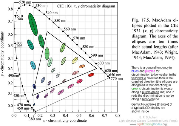
If one plots small color differences that are just noticeable in various directions in the CIE (xy) diagram, the differences fall into an ellipsoid instead into a circle. This means that two colors can be very far apart in, e.g., the green region of the diagram before they appear to change color. In contrast, in the blue region, the same perceptual difference occurs over a much smaller distance. The realization that constant chromaticity differences would not yield constant perceived color differences led to development of multitude of color spaces, one of which has a dominant place in CIE colorimetry - CIELAB color space. More about it later.
Another, and more practical way to arrive to the horshoe diagram is to convert color matching functions to chromaticity (x,y) coordinates (eq. II) and plot the values in Excel spreadsheet. In this example, tristimulus value X is equal to the component [x] of color matching function. Analogously, Y and Z components equal to [y] and [z], respectively. It is important not to mix the color matching functions for different observer (CIE 1931, 2o, CIE 1964, 10o). For details, see the formulas in "cie-xy" tab of this spreadsheet. Charts in Fig. 5 were created using VB macros included with this spreadsheet.
(top)↑ Light Sources and Illuminants:
Terms such as reflectance and spectral radiance are used to describe the optical properties of materials and light sources. Reflectance (a measure of reflected light) depends on many parameters such as thickness of the sample, surface, angle of light incidence, spectral composition of the radiant source, and polarization effects. Both light sources and surfaces are described by their spectral power distribution (SPD) that contains all the basic physical data about the light and serves as the starting point for quantitative analyses of color. From the SPD, both the luminance and the chromaticity can be derived to describe color in the CIE system. For the reflective objects, the tristimulus color specification (CIEXYZ) is dependent on the viewing illuminant described by its SPD. Color of an emissive light source is also described by its unique CIEXYZ values. In contrast to light sources, reflective surfaces do not have intrinsic color although tristimulus XYZ values can be ascribed to the light reflected from them under a specific illuminant.
The CIE standards committee made a clear distinction between the terms illuminant and source. Source refers to a physical emitter of light, such as lamp, monitor, or the sun. Illuminant refers to a spectral power distribution, not necessarily provided directly by a source. As mentioned in the previous section, any color of physical light can be expressed by the chromaticity coordinate (x, y) on the CIE 1931 (x, y) chromaticity diagram (Fig. 2).
Blackbody radiator:
Technically, any object at any temperature above the absolute zero (0 K) will emit and absorb electromagnetic radiation to some extent. The intensity and frequency distribution of the radiation depends on the detailed structure of the body. A black body is a theoretical object that is capable of emitting and absorbing all frequencies of electromagnetic radiation uniformly (resulting in continuous spectra). A good approximation to a black body is a pinhole in an empty container maintained at a constant temperature. Such bodies do not emit light, and therefore appear black if their temperatures are low enough so as not to be self-luminous (black body is completely black at temperature of absolute zero while still having a ground state vibrational energy a.k.a. zero-point energy). At high temperatures (> 1,500 K) an appreciable proportion of the radiation is in the visible region of the spectrum.
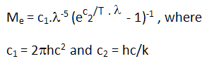
As a result of established equilibrium (by emitting and re-absorbing radiation energy), emission spectrum of the black body is determined only by its temperature. In practice no material has been found to absorb all incoming radiation. The equation describing the specific intensity emitted by a "black body" at a given wavelength as a function of temperature is known as Planck's law for the black body radiation. The mathematical function describing the shape is called the Planck function (eq. III).
 (III)
(III)Other parameters are: λ = wavelength (m), T = temperature (K), h = Planck constant (6.62607E-34 J.s), c = velocity of light (299,792,458 m/s), and k = Boltzmann constant (1.38065E-23 J/K). Resulting spectral radiant exitance per unit wavelength interval Me(λ) is in units of W . m-2 . nm-1. Normalizing values of Me(λ) to unity (dimensionless) at λ=560 nm leads to Relative radiant power, which is often used in many graphical representations of spectral distribution (Fig. 3). Planckian blackbody calculation is demonstrated in this spreadsheet together with calculation of tristimulus XYZ values for blackbody radiator.
| Figure 3: Relative spectral distributions of radiant exitance of blackbody. |
|---|
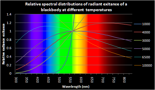 |
Regions of invisible radiation are shown in black. the above referenced spreadsheet allows for calculations of relative radiant power (dimensionless) and total radiant exitance (W . m-2) at a given temperature. Inspect formulas in the corresponding cells to uncover math behind graphs in Fig. 3.
| Figure 4: Daylight (D65, D50) and blackbody radiators |
|---|
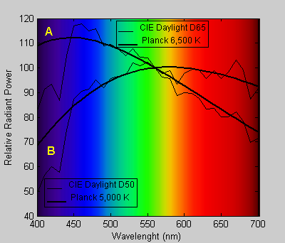 |
Deatails of continuous spectrum of blackbody light in comparison to two standard CIE daylight illuminantsis are shown in Fig. 4 (thicker black lines). Since the temperature of a blackbody radiator describes its complete spectral power distribution and thereby its color, it is commonly referred to as the color temperature of the black body and as such it can be expressed by the chromaticity coordinates (x, y) on the CIE 1931 (x, y) chromaticity diagram, as shown in Fig. 5. The trace of the chromaticity coordinates of a blackbody plotted near the center of the diagram is the so-called Planckian locus (Fig. 5). The colors around the Planckian locus from about 2,500 to 20,000 K can be regarded as the source white: 2,500 K being reddish white and 20,000 K being bluish white. The point labeled "A" (illuminant A) is the typical color of an incandescent lamp (CCT 2,856K) and illuminants D50 and D65 are the typical colors of day light, as standardized by the CIE. The color shift along the Planckian locus (warm to cool) is visually acceptable for general lighting, while color shift away from the Planckian locus (greenish or purplish) is perceived as unnatural. Strictly speaking, color temperature cannot be used for color chromaticity coordinates (x, y) off the Planckian locus, in which case the correlated color temperature (CCT) is used. CCT is the temperature of the black body whose perceived color most resembles that of the light source in question. Due to the perceptual non uniformity of the CIE (x, y) diagram, the iso-CCT lines are not perpendicular to the Planckian locus on the (x, y) diagram (Fig. 6).
| Figure 5: CIE 1931 (x,y)-Chromaticity Diagram |
|---|
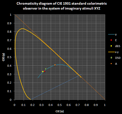 |
Figure 6: Correlated color temperature isotherms

To calculate CCT, another improved chromaticity diagram (Uniform-chromaticity scale CIE 1960 (u-v) diagram - now superseded by CIE 1976 (u'-v') diagram) is used, where the iso-CCT lines are perpendicular to the Planckian locus.
As mentioned earlier, the CIE has defined several standard illuminants for the use in colorimetry. To represent different phases of daylight, a continuum of daylight illuminants has been defined by the CIE, which are uniquely specified in terms of their correlated color temperature (CCT). The D65 and D50 illuminant spectra are two daylight illuminants commonly used in colorimetry, which have CCTs of 6,504 K and 5,003 K, respectively (Fig.3). Spectral power distribution of the D65 source has clearly more of the blue component of the visible spectrum while the D50 source would appear reddish. The CIE Illuminant A represents a blackbody radiator at a temperature of 2,856 K and closely approximates the spectra of incandescent lamps. For links and references, go here.
Summary:
- Black body is a theoretical object that when heated to a high temperature will emit visible light. Spectrum of this light can be theoretically predicted from the Planck's law.
- Chromaticity (color) of the light emitted over a range of temperatures will be perceived as a "white" (bluish, yellowish or reddish). Perceived "white" color is commonly referred to as the color temperature of the black body.
- The trace of the chromaticity coordinates of a blackbody radiator plotted inside the CIE (1931) xy chromaticity diagram is called Planckian locus.
- Correlated color temperature (CCT) is the temperature of the black body whose perceived color most resembles that of the light source in question. Chromaticities falling on the Planckian locus always have true color temperature while chromaticities near the locus have only correlated color temperature.
- Chromaticity of a light source cannot be described by CCT only. Information on how far off the locus our chromaticity values are is as important as the CCT.
- In most cases, where a "color temperature" is stated for some light source, it is almost always the CCT. Also for the CIE defined chromaticities of standard illuminants/sources, reference should always be to a CCT since these sources are not true blackbody radiators.
- In practice, monitor calibration can be always targeted at either Planckian or CCT temperatures. We just need to select chromaticity of the desired "white".
Chromatic Adaptation:
Let's start the topic of chromatic adaptation with a few examples. Suppose we have a white piece of paper that we look at under three different lightning conditions: midday, late sunset and at home under incandescent light. While all three light sources (illuminants) have different spectra and appearance (bluish, yellowish and yellow-reddish, respectively), color of the white paper that we perceive is very similar, i.e. white. This experiment works best if one looks only at the piece of paper without any background. Similarly, perceived differences in a tint of monitor that is calibrated to D50 (yellowish) versus D65 (bluish) will be less apparent in about 10 seconds (though it may take a few minutes to completely adjust). The effect is more pronounced when monitor is observed without any external reference object (painted walls, gray or black frames of your monitor). This is because our visual system adapts to the illuminant (the chromaticity of the illumination source) by shifting the appearance of all colors to restore the neutral appearance of a white surface. This phenomenon is known as the color constancy ![]() of human vision.
of human vision.
One of the mechanisms for color constancy is chromatic adaptation which can be defined as the ability of the human visual system to adjust to changes in the color of illumination. Preceding two examples suggest that chromatic adaptation is a result of sensory adaptation as well as cognitive behavior. The cognitive component of chromatic adaptation process is also known as discounting the illuminant and depends on observer's knowledge of scene content.
From the digital photography stand point, more general conclusion could be formulated such that any color space transformation is dependent on the source and destination illuminants. In other words, to achieve the same visual appearance of the original image under different display conditions (such as a computer monitor or a light booth), the captured image tristimulus values have to be transformed to take into account the light source of the display viewing conditions. Such transformations are called chromatic adaptation transforms (CATs). Thus, applying a chromatic adaptation transform to the tristimulus values (X,Y,Z) of a color under one adapting light source predicts tristimulus values (X',Y',Z') of the corresponding color under another adapting light source. Corresponding color refers to two stimuli that might have different XYZ tristimulus values, but because of chromatic adaptation to both illumination sources, they might appear to match. To be completely clear, CAT does not predict the colorimetric (XYZ) values of an object when illuminated by the destination source!! It is all about appearance of the corresponding color, not the absolute match of tristimulus values. Basic CIE tristimulus colorimetry is not designed to predict matches across different viewing conditions. Chromatic adaptation transforms thus extend basic tristimulus colorimetry. However, it is important to recognize that chromatic adaptation can only deal with small variations in the color of the illuminant. For huge changes in the color of the light source, we would surely see a change in the color of the object.
Common white-point chromaticities for a computer monitor are D50, D65, or D93 (CRTs). The "native white point" of common LCD monitors is around 6,000 K. Photographic printed outputs are usually evaluated under a standard illuminant of D50 (light boxes). The profile connection space (PCS) as defined by International Color Consortium (ICC) is D50, resulting in each device profile mapping image colors from source specific illuminant (e.g. CCT 6,000 K or D65 for monitors) to D50 illuminant.
There are numerous methods described in color textbooks developed for the chromatic adaptation. Many such transforms are based on the underlying model of chromatic adaptation proposed by von Kries. This model states that the individual sensors in the human eye are independent of the other and each type is adapted according to its adaptation function. Experiments indicate that a significant part of chromatic adaptation appears to take place in the photoreceptors, either as a change in the individual sensitivity curves of the L (long wavelengths), M (medium wavelengths) and S (short wavelengths) cones, or in the response of the retinal secondary cells to the cone outputs. To model this process in a meaningful way, it is necessary to transform from CIE XYZ tristimulus values into LMS cone responses. The cone responses under two illuminants can be described by a linear transform.
Mathematically the von Kries model can be written as:
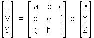 |
(IV) |
where coefficients at the diagonal of the 3 x 3 matrix (a, e, i) are the independent gain control factors. How these gain control coefficients are calculated is the key aspect to most CAT models. When transformation (IV) is performed in CIEXYZ space or RGB space (as opposed to the LMS cone space) it is referred to as an XYZ scaling or a "wrong von Kries" transformation (V). Symbols D and S denote a pair of destination and source illuminants and the diagonal matrix is composed of ratios of source and destination illuminants. Such a simple scaling by diagonal matrix can be also applied to the RGB -> XYZ transfer matrix C (see below eq. XI) to ensure the white point preservation.
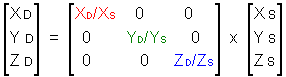 |
(V) |
A more general model of chromatic adaptation (based on the von Kries model IV) is the so called generalized linear model (VI). In this case chromatic adaptation is once again controlled by independent gain factors (diagonal matrix D), but this time, D operates not on the tristimulus values but on a linear combination of vision system's sensors (cone responsivities):
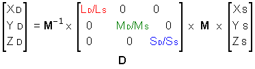 |
(VI) |
M is a 3x3 matrix that transfers the source tristimulus values to three cone responsivities Ls, Ms, Ss as per IV. This source cone responsivity is then converted to destination (Ld, Md, Sd) by a diagonal matrix D containing the destination-to-source ratios of the cone responsivities (such as Ld/Ls, Md/Ms, Sd/Ss). Coefficients of the diagonal matrix D are determined from the tristimulus values of the source and destination illuminants (denoted by W) and the matrix M as follows:
[ Lw,s Mw,s Sw,s ]T = M * [ Xw,s Yw,s Zw,s ]T and [ Lw,d Mw,d Sw,d ]T = M * [ Xw,d Yw,d Zw,d ]T
By dividing the destination and source responses, we obtain: D = diag( Lw,d/Lw,s , Mw,d/Mw,s, Sw,d/Sw,s )
Last step is to convert the destination cone responsivities to the new tristimulus values:
[ XD YD ZD ]T = M-1 * [ L d M d S d ]T
Finlayson et al. have shown that matrix M can be used to transform either the cone or tristimulus values into a suitable RGB space. In this case, the diagonal matrix D is composed of the white points of two illuminants in the RGB space.
From the practical point of view, the most commonly used transformation is the so called Bradford chromatic adaptation transform. Analogously to the above described CAT, it consists of a 3 x 3 linear transform from XYZ tristimulus values to an optimized set of Ls, Ms, Ss responses. These cone response values are then scaled to the Ld, Md, Sd values for the illuminant (or chosen white point) using a simple von Kries normalization. Specific feature of the Bradford transformation is the adaptation-dependent exponential function applied to the short wavelength cone signal (blue channel). The red (L) and green (M) domains remain strictly linear. However, in many applications, blue channel non-linearity is neglected. The Matlab code for both versions of the Bradford CAT is shown below (bradford.m). For simple spreadsheet form, download this Excel file. Practical use of the Bradford transform involves multiplication of the transform matrix by the source tristimulus values as in eq. (VI).
% bradford.m
% calculates Bradford matrix from source to destination illuminant

Mcat = [0.8951 0.2664 -0.1614;
        -0.7502 1.7135 0.0367;
        0.0389 -0.0685 1.0296];

% destination white (here D50)
D50 = [96.4220  100.0000   82.5210];

% enter tristimulus of the source white (e.g., monitor)
DXX = [95.105 100.000 108.548];


sxx = Mcat * DXX';  % source cone responses
d = Mcat * D50';    % destination cone responses
tau = (sxx(3)/d(3))^0.0834; % S-cone non-linear correction


diag = [d(1)/sxx(1) 0 0;  % diagonal linear matrix
        0 d(2)/sxx(2) 0;
        0 0 d(3)/sxx(3)];

diag_nl = [d(1)/sxx(1) 0 0;
             0 d(2)/sxx(2) 0;
             0 0 (d(3)/sxx(3)^tau)*sxx(3)^(tau-1)]; % non linear coeff in S

Mbfd = inv(Mcat) * diag * Mcat;       % "linear" Bradford CAT matrix
Mbfd_nl = inv(Mcat) * diag_nl * Mcat; % "non-linear" Bradford CAT matrix

disp ('Bradford Matrix:'                )
disp (Mbfd)
disp ('Bradford Matrix nonlinear:'                )
disp (Mbfd_nl)
Bradford transform is implemented as the only CAT in Adobe Photoshop.
Summary:
- Colors change their appearance upon changes in the color of the light source.
- Chromatic adaptation is the ability of the human visual system to discount the color of the illumination and to approximately preserve the appearance of an object.
- Chromatic adaptation transforms (CATS) seek to best model how the same color appears under two different lightning conditions (illuminants). CAT is a method for computing the corresponding color under a reference illuminant for a stimulus defined under a test illuminant.
- Due to its good performance, the Bradford CAT is recommended for appearance transformations from one illuminant to another.
- Such transformations are needed when comparing colorimetric data obtained at or referenced to different illuminants (light sources). Examples may include comparison of color patches on monitor having different color temperature, referencing colors to a standard illuminant (D50), or matching the monitor and light box light sources.
Transformation of RGB Primaries:
With many imaging devices being additive systems of red, green and blue colors, RGB primaries are well suited for colorimetric calculations. Those devices include, for example, digital cameras, scanners, projectors, and LCD/CRT displays. Moreover, since CIE color-matching functions are linearly related to RGB primaries, there is a simple relationship between RGB and CIEXYZ coordinates. In the 3-D coordinate space, one conveniently uses matrix algebra to do all the necessary conversions (for basics, look here - Introduction to Matrix Algebra from Autar K. Kaw : e-book and also download this great Excel add-in).
Let's start with few assumptions commonly used in colorimetry, namely proportionality and additivity of the color stimuli that are used in additive color mixing.
Lλ,mix = r . Lλ,red,max + g . Lλ,green,max + b . Lλ,blue,max
where r,g,b are relative amounts of the respective light.
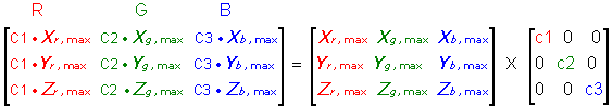
X = R . Xr,max + G . Xg,max + B . Xb,max
Y = R . Yr,max + G . Yg,max + B . Yb,max (T-1)
Z = R . Zr,max + G . Zg,max + B . Zb,max
Now, we have just shown that the digital device RGB coordinates can be transformed to visual tristimuli using a system of linear equations (T-1). In this system, R, G, and B are independent variables and X, Y, and Z are the dependent variables. Following the matrix notation, transformation (VII) is generally used to calculate the XYZ coordinates of pixels displayed on the monitor :
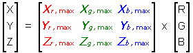 |
(VII) |
Equation (VII) essentially performs a linear operation that converts between two 3-dimensional spaces, in our case RGB and XYZ (see the side panel for graphical representation of such transformations).
In even more general form, [XYZ]T = [3x3 matrix] x [RGB]T (superscript "T" denotes the transpose of the matrix). The middle [3x3] matrix (so far unknown) is derived from chromaticity coordinates of the RGB primaries and coordinates of the adapted white point. For example, for sRGB (D65) color space, the matrix is following:
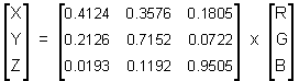 |
(VIII) |
Note that the sum of the row coefficients in eq. (VIII) equals to the XYZ coordinates of the white illuminant (in this case D65 ![]() ). This follows from the eq. (VII) for a special case of R=G=B=1, that is, a white light. To calculate just the luminance (Y), the following simplified equation can be used:
). This follows from the eq. (VII) for a special case of R=G=B=1, that is, a white light. To calculate just the luminance (Y), the following simplified equation can be used:
Y = [Yr,max Yg,max Yb,max] * [RGB]T (vector of the Y values comes from the second row of the [3x3] matrix).
In case that we know the XYZ coordinates and need to calculate the coresponding RGB values, the [3x3] matrix has to be inverted and the following equation (VIII-inv) used.
 |
(VIII-inv) |
To practice on a real example, let's calculate the R'G'B' values of the red patch of the GretagMacbeth ColorChecker. We will assume the sRGB color space and use the provided D65 L*a*b* values. The L*a*b* values for this particular patch (L* = 40.554, a* = 49.972, b* = 25.45) were reported by the GretagMacbeth and are also part of the Imatest software. First, we need to obtain the XYZ values from the L*a*b* values. In this case we need the D65 XYZ values (because the sRGB color space is D65) and thus no chromatic adaptation will be needed. Conversion from the L*a*b* values to the XYZ can look rather complicated, but can be easily achieved by using a spreadsheet.
% Lab to XYZ (Matlab style) # for L* > 8.0
X = Xn*(((L*+16)/116) + (a*/500))^3;
Y = Yn*((L*+16)/116)^3;
Z = Zn*(((L*+16)/116) - (b*/200))^3;
In this case, the Xn,Yn,Zn values correspond to the standard illuminant of the chosen color space (sRGB D65)
Xn= 0.95047
Yn= 1.00
Zn= 1.08883
In this example, we will calculate the blue component (Z) of the red ColoChecker patch:
Z = 1.08883 * (((40.554 +16)/116) - ((25.45/200))^3 = 0.0509
The corresponding red and green values are: X = 0.1927, Y = 0.1159. The complete XYZ matrix is then:
[0.1927
0.1159
0.0509]
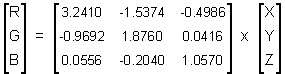
And now the matrix multiplication. From the matrix algebra, it is known that two matrices A and B can be multiplied if the number of columns of A is equal to the number of rows of B. Number of columns in eq. VIII-inv is 3 and so is number of rows in the preceding XYZ matrix. Thus we can multiply both matrices. In this part, we will calculate the R component of the RGB triplet:
R = 0.1927*3.2406 + 0.1159*(-1.5372) + 0.0509*(-0.4986) = 0.4210
G = 0.3280 and B = 0.0409 are calculated similarly.
Now, we are almost done. However, since we used a linear transformation of XYZ values, we obtained the linear RGB values. The linear RGB values need to be transformed to nonlinear (gamma encoded) values via the gamma correction, having a gamma 2.4-1 , an offset 0.055, and a slope of 12.92 (standard sRGB encoding). Finally the sR'G'B' values are scaled to 8-bit integers by multiplication with 255. We will demonstrate the calculations by a pseudo-code:
if RGB(i) <=0.004045
R'G'B'(i) = 12.92*RGB(i)*255;
else
R'G'B'(i) = (1.055*RGB(i)^(1/2.4)-0.055)*255;
For the red component: R = (1.055*0.4210^(1/2.4)-0.055)*255 = 174
G = 51 and B = 57.
In conclusion, the L*a*b* values of the red patch (L* = 40.554, a* = 49.972, b* = 25.45) have the correspong R'G'B' values of 174, 51, 57 in the sRGB color space.
Now the challenge comes. When characterizing a display (as an example), we would not necessarily be dealing with standard radiation source of a known color temperature, not mentioning the uncertainty in values of the RGB primaries of our display and its gamma correction. Hence, the above sRGB 3x3 matrix (VIII) won't be any good for our work.
Well, how do we get the right matrix coefficients and how can we use the above equations? Reasonable point to start is to assume complete spectral proportionality of our monitor. This means that if each RGB channel has scalable spectra, its chromacities will not vary with the lightness level. If this assumption holds up, the use of eq. (VII) is justified - as long as the additivity is also preserved. We will make the latter assumption as well. This additionally means that the tristimulus values for the display white are at least very close to the summed tristimulus values of the full-on red, green, and blue primaries.
Now, to get the corresponding XYZ coordinates of primaries, a simple measurement of red, green, blue, and white patches on our display will be required. Why the white patch? Besides checking the additivity, we also have to determine the white point of our display. This is important for correct CAT transform from monitor white to any standard state of defined source, say D50 (which is conveniently the ICC standard for profile connection space ). For this purpose, we will apply Bradford chromatic adaptation transform (CAT) on our measured XYZ data.
There is one more step to check. Due to the various errors connected to measurements, least square estimation of the matrix coefficients, or quality of the display circuitry, there is a good chance that our [3 x 3] matrix is not white point adapted (i.e., the additivity rule does not hold well). This means that RGB to XYZ conversion (for R=G=B=1) would not result in expected coordinates of the white at D50 (0.964212, 1.00000, 0.825188). In such a case, correction to the XYZ primaries in the matrix has to be done. Only then the sum of the row coefficients will be equal to the XYZ coordinates of the white illuminant (in this case D50). Just to clarify - this is not a chromatic adaptation transform - that one is done on XSYSZS/XDYDZD values and corresponds to an appearance transform (see above). Required white point adaptation is purely mathematical scaling by a diagonal matrix that again ensures correct tristimulus values of the destination "white" and the corresponding neutral gray. We have already seen one example of XYZ scaling (a "wrong von Kries") in transformation (IV) in the previous paragraph. It may not be immediately apparent, but multiplication by a diagonal matrix results in a matrix where each column is multiplied by the same coefficient from the diagonal. In our specific case of RGB to XYZ transfer matrix, tristimulus triplet defining each of the RGB channels is multiplied by a coefficient such that the sum of rows will correspond to [XYZ]T vector of the white point (IX). In general, consequences of XYZ scaling by a factor are following: i) x,y chromaticity values do not change (as per (II)), ii) CCT of the white point will not change, iii) L*a*b* and RGB values are, however changed. Since XYZ to L*a*b* conversion formula contains a white point scaling, for R=G=B=1, L* = 100, a* = b* = 0.
 |
(IX) |
Let's first see how we obtain this diagonal matrix. As we recall from the first paragraph, XYZ values can be transformed into x,y,z chromaticity values using eq. (II). Substituting into eq. (VII), we get a new equation (X). Now, if you are wonderings how the second row of the 3x3 matrix in (X) came about, here is the trick: Yr = yr * Yr/yr. Now, let's take out the Yi/yi and make them equal to Ti (i = r,g,b). In the resulting eq. (XI), colorimetric RGB primaries (C) are related to tristimulus values via additional "corrective" matrix (T). This relationship is in agreement with the formula recommended by Xerox Corp. (as per "Color Encoding Standard", C-3 (1989)).
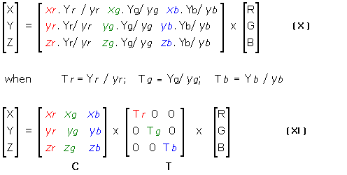 |
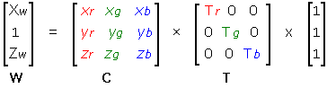
Coefficients (xr, yr, zr), (xg, yg, zg), and (xb, yb, zb) in (XI) are the chromaticity coordinates of the red, green, and blue primaries, respectively. New parameters Tr, Tg, and Tb are the proportional constants for the corresponding primaries under the adapted white point (that's the correction we need). Equation (XI) can be solved for [T] using a known condition of a gray-balanced and normalized RGB system (i.e., for R=G=B=1, a reference white point - in our case D50 - should be produced). Normalized tristimulus values of the D50 white point [W] = [0.964212, 1, 0.825188]T are used together with known coordinates of primaries to calculate [T] = [C]-1 [W] from eq. (XI).
 |
(XII) |
Resulting T values are substituted back into eq. (XI) with the known chromaticity coordinates of primaries. Now, we know [C] and [T] that can be combined into one transfer matrix [M]. Final transformation is then of the form of:
[XYZ]T= [Mwp] x [RGB]T
To help you with the above calculations of matrix [Mwp], here is the Excel spreadsheet for download. Below is the Matlab code.
% WP_adapt.m
% Reads manually provided 3x3 matrix and
% returns RGB2XYZ conversion matrix adapted to a white point

clear all

Tm = [48.2793   32.1731   14.4443;
      25.9368   65.8478   10.5637;
      1.1492    8.1183    74.8447]'; % enter the 3x3 matrix, transpose;

W=[0.964212; 1; 0.825188]; % XYZ of the white point (here D50)


% Build xyz chromaticity matrix
xyz=[Tm(1)/sum(Tm(1,:)), Tm(1,2)/sum(Tm(1,:)),Tm(1,3)/sum(Tm(1,:));
    Tm(2)/sum(Tm(2,:)), Tm(2,2)/sum(Tm(2,:)),Tm(2,3)/sum(Tm(2,:));
    Tm(3)/sum(Tm(3,:)), Tm(3,2)/sum(Tm(3,:)),Tm(3,3)/sum(Tm(3,:))]';


T = inv(xyz) * W; % Proportional constants for R,G,B
Tc = [T(1) 0 0;0 T(2) 0;0 0 T(3)]; % 3x3 Matrix of proportional constants
MD50 = (xyz * Tc); %Final RGB2XYZ matrix for the white point Tm

format short

%-----------Display---------%
disp ('Original matrix: ')
disp (Tm')
disp ('M adapted to D50 (MD50): ')
disp (MD50.*100)
Unfortunately, there is one more complication in the matrix transformation. All the above equations work fine when radiant output at R=G=B=0 is equal to zero. For non zero output at the black, a correction has to be made to the matrix to account for this "flare" component. This phenomenon is quite common for LCD monitors (link) and cannot be avoided as the liquid crystals pass some light through even at the "switched-off" state. Typical [3x3] matrix is then extended to a [3x4] matrix by adding the black-level radiant input Xk, Yk, and Zk (XII). This form of the matrix ensures that values for the black output are added to the resulting XYZ values at the dark levels while the bright values will be corrected proportionally by only a fraction of the black values. Values at the highest output (R=G=B=1) will not be corrected at all.
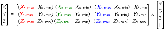 |
(XIII) |
In order to calculate radiometric scalars (linearized RGB values) from the measure XYZ values and RGB primaries, the inverse black corrected matrix should be used (XIV).
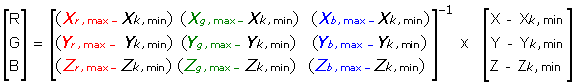 |
(XIV) |
Note the last two equations as we will use them extensively in display characterization examples.
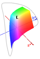
CIELAB color space:

Color differences:
Links: GamutVision - Koren Norman
Links and References:
Following are books that I would recommend reading.
Colorimetry :
- Wyszecki, G., Stiles, W. S., Color Science: Concepts and Methods, Quantitative Data and Formulae, Wiley-Interscience; 2nd Edition (2000).
- A review of RGB color spaces by Danny Pascale.
- Berns, R.S., Billmeyer and Saltzman's Principles of Color Technology, 3rd Edition, Wiley-Interscience; (2000).
- Poynton, C., A Guided Tour of Color Space, web document (1997).
- Digitalcolour.org (links to many useful topics and programs)
- CIE XYZ.pdf (Douglas A. Kerr)
- Colour4free (pdf) (Putting numbers to colour: CIE XYZ)
- Color Representation (pdf) Department of Computer Science at the University of Haifa
- HSL(uv) color space. Alexei Boronine
Light sources and Illuminants:
- Light and the Eye on Correlated color temperature by Bruce MacEvoy (lots of details)
- Color Temperature by Douglass A. Kerr - clear and easy to read article
- "White Point" at Wikipedia
- Blackbody radiation spectra
Chromatic Adaptation Transforms:
- Kang, H.R. , Computational Color Technology, SPIE Press, Bellingham, Washington USA (2006).
- Ssstrunk, S. and Finlayson, G.D., Evaluating Chromatic Adaptation Transform Performance, Proc. IS&T/SID 13th Color Imaging Conference, pp. 75-78, 2005.
- Finlayson, G.D. and Ssstrunk, S., Spectral Sharpening and the Bradford Transform, Proc. Color Imaging Symposium (CIS 2000), pp. 236-243, 2000.
- Süsstrunk, S., Holm, J. and Finlayson, G.D., Chromatic Adaptation Performance of Different RGB Sensors , Proc. IS&T/SPIE Electronic Imaging 2001: Color Imaging, Vol. 4300, pp. 172-183, 2001.
- Süsstrunk, S., Buckley, R. and Swen, S., Standard RGB Color Spaces, Proc. IS&T/SID 7th Color Imaging Conference, Vol. 7, pp. 127-134, 1999.
- Sharma, G., Understanding Color Management, Thomson Delmar Learning (2004), pp. 86-88.
- Johnson, G. M., Fairchild, M. D., Digital Color Imaging Handbook (Electrical Engineering & Applied Signal Processing Series), Sharma G. (Ed.), pp.115-171, CRC, (2003).
- Wandell, B.A., Silverstein, L.D., Digital color reproduction, The Science of Color, pp.281-316 (2003).
Transformations of RGB Primaries:
- Poynton, C., Colour Space Conversions
iPython (Jupyter) Notebooks:

RGB colorspace
Corresponding XYZ
color space
Corresponding xyY
color space
Transformation to L*a*b*
