

Contents:
1. Examples of a Display Characterization:
Over the past few years, I have worked with Samsung SyncMaster 191T and later with Eizo CG19 LCD monitors, both connected to DVI-D output on my video card (MSI GeForce 6800 GT NX6800GT-TD256). With such a setup, the display receives 8-bit digital signal from the video card. In case of the SyncMaster 191T LCD, don't be surprised if contrast and RGB adjustment options are grayed-out in the monitor's OSD (on-screen-display). Should you have chosen the analog output from the video card (15-pin analog VGA), access to all OSD option, including the R, G, B controls would be available. Eizo CG19 monitor has a built in 10-bit LUT that completely controls the monitor. Additional adjustment in the video card LUT is possible, but not necessary. With this video card and CG19 display, one has the so called "8-10-8-bit" monitor system. 8-bit signal sent out from the computer is then given 256 ideal tone selections from the 10-bit (1,021 tones) LUT in the monitor. Such a setup increases the gamma compensation accuracy and results in smoother gradients than 8-bit video card LUT would provide.
Read more on monitor adjustments:
SyncMaster 191T LCD display: at the time of its release (2002), it was a general purpose although a higher-end monitor. It was based on PVA LCD TFT matrix produced by Samsung (panel LTM190E1). It has the native resolution of 1280 x 1024 pixels. Manufacturer declares brightness of 250 cd/m2, contrast ratio of 500:1, and response time of 25 ms. The brightness is controlled through modulation of power of the fluorescent backlight lamps. Over the years, I realized that response time was not that great while colors were acceptable. Contrast was indeed very good. Some light seepage was clearly visible at the left lower side.
Eizo CG19 LCD display: is a monitor specifically intended for professional work with color and features excellent color management capabilities. It is based on DD-IPS LCD TFT matrix produced by Hitachi (panel NL128102BC29-01). It has the native resolution of 1280 x 1024 pixels. Manufacturer declares brightness of 280 cd/m2, contrast ratio of 450:1, and excellent response time of 20 ms. The brightness is controlled through modulation of power of the fluorescent backlight lamps at 170 Hz. As with other IPS matrices, a violet hue appears in black colors when viewed from a side. Contrast is somehow low, but viewing angle and color are excellent.
(top)↑1.0. Characterization of the Eizo CG19 display:
This example discusses characterization of the calibrated display. Since we only characterize the current calibration or just the current monitor state, neither icc profiles nor the color management is needed. Predefined R'G'B' values are sent directly to the monitor (video card) and the output values are measured by colorimeter or spectrophotometer. Since the experimental output values are known (device readout), the remaining part of the characterization process is to find out what are the theoretical (reference) values of the colors sent to the monitor. Several methods for finding these reference values are discussed in this section. The concept of characterization was introduced in the section of "Colorimetric Characterization". For other methods of monitor characterization, read the Appendix B in the PatchTool manual at the BabelColor web site. In this example, the Eizo CG19 LCD display was calibrated using Argyll CMS and X-Rite colorimeter DTP-94. Calibration is described in other section of these pages. Target parameters were set to gamma = 2.2, brightness = 120 cd/m2 and CCT = 6,500 K. As mentioned earlier, this particular monitor is equipped with 10-bit LUT and thus it would make more sense to calibrate it in its own monitor LUT to improve smoothness of gradients and quality of grayscale. This option will be described later. For now, we will evaluate calibration done by Argyll CMS. Methods described here apply to any calibrated monitor regardless of calibration technique used.
First, a few words on the data collection.
- Ambient light:
- Test images:
-
Measurements were taken under controlled lightning conditions, in this case, a completely darkened room. Any flare resulting from the display was corrected for in the model. The white point of the display was transformed to CIE D50 source using Bradford chromatic adaptation transform. All calculations assumed the CIE 1931 2o standard observer.
-
Square color or grayscale patches were displayed in the center of the LCD display. Background of the display was set to mid-gray (RGB=128). The "Measure Tool" module from the ProfileMaker 5
suite of software or the 'dispread' utility of the Argyll CMS were used to
display and read the patches.
You can download the LOGO and .ti1 formatted files for RGB ramps, color patches and gray patches by following these links:
To run them, place the PM5 files into
C:\Program Files\GretagMacbeth\ProfileMaker Professional 5.0.8\Reference Files\Monitor folder
and select them (one at the time) from the program menu (see details in section ProfileMaker).
To use the dispread utility follow the examples at the Argyll CMS section. In Argyll CMS, simply issue the following command
to display and read the ramp file.
C:\CMS\bin>dispread -K -yl data\RGB_ramps161As long as we are an the topic of "Test Images" (quite unreletaed to the above), following are links to jQuery script that will display & animate supplied gray or color patches through the web browser window. Patches are both untagged and tagged with several common icc profiles to allow for assessment of color management of any particular web browser.
-
The input ramp data set consists of the RGB steps ranging from 0 to 255 per channel in increments of 5. This gives us 51 steps per channel (153 data points). Black and white patches were measured four times each and the corresponding tristimulus XYZ values were averaged.
All 161 patches were displayed on the monitor and their colorimetric values measured using the X-rite DTP-94 colorimeter or the EyeOne Pro spectrophotometer. The input set of color patches consists of 31 gray steps ranging from 8 to 247 in increments of 8. Black and white patches are the same as in the case of ramps. Six patches of R,G,B,C,M,Y colors follow with the remaining 116 patches generated by Argyll's 'targen' utility. The input set of gray patches consists of 53 gray steps ranging from 0 to 255 in increments of 5. Black and white patches are again averaged. The measured tristimulus values are normalized so that the Y value of the white point (RGB=255) is equal to 100. This corresponds to multiplication of each XYZ component by a luminance factor f = 100/average(Yw1:Yw4). Remember, scaling all three tristimulus components of the data set by the same factor does not change the color. To make all the measurements consistent, all conversions from RGB to XYZ use [3x4] matrix MD50 (eq. XIII). This matrix is derived from the display RGB primaries chromatically transformed to D50 source and rescaled to match the D50 white point.
The final output is average CIEDE2000 difference between the measured and predicted values for the whole data set. Since CIEDE2000 evaluates differences in the L*a*b* color system, this method should provide more realistic results as the measure is done in perceptually uniform domain.
- Using the Babecolor CT&A:
- Enter (x,y)-chromaticity coordinates of the white point ( the XYZ values at R=G=B=255) into the Bruce Lindbloom's CIE Calculator (row xyY, Y=1) and click the button on the left of the same row. Read the CCT from the row "Color Temp." and record it somewhere for the later use (e.g. 6,450 K).
- In the BabelColor CT&A, create a "Custom RGB space" with CIE (x,y)-chromaticity coordinates of the RGB primaries (obtained from the RGB ramp measurement). CIE (x,y)-values can be calculated as follows: x=X/(X+Y+Z), y=Y/(X+Y+Z)
- Setup a custom white point in the Temperature section (here "Black body" 6,450 K)
- Save as a Custom Space (e.g. CS64). By doing the above, several otherwise lengthy tasks were achieved. First, the chromatic adaptation transform matrix (Bradford) was calculated for you. Second, RGB to XYZ [3x3] matrix was also calculated for you.
- Excel processing *: Download the corresponding Excel spreadsheets "Ramps_XYZ.xls", "Patches_XYZ.xls", or "Gray_XYZ.xls", respectively. These spreadsheets were written to process the measurement data and to calculate CIEDE2000 color difference values for each patch including the average DE2000, ΔH, L*a* b* coordinates and much more. Instructions are included in the Excel file. These spreadsheets can be also used to output experimental data that is used in GammaCalc section of these web pages. Nonlinear fit is implemented to predict the display gamma from your own data.
- For simple extraction of measurement data from any LOGO or CGATS formatted file, use scripts at this web page. Such files are typically created by ProfileMaker 5, Argyll CMS, and BabelColor PatchTool applications.
Now, let's assume that we have run all the patches and recorded the corresponding tristimulus data. Having all the data available, we can determine the main colorimetric parameters, namely the tristimulus coordinates of the display RGB primaries, the white point, gamma, and the conversion matrix. In addition, the data for each RGB ramp will allow us to verify the constancy of primaries and their additivity. We will also assess the accuracy of reproduction of the digital version of the GretagMacbeth ColorChecker.
Before we can start comparing the measured and expected values of the color patches, there is one additional task to do - we need to obtain the corresponding "theoretical or reference" XYZ (or L*a*b*) values of the displayed R'G'B' patches. These would be the device-independent values corresponding to the R'G'B' values sent to the monitor during measurements. They are either estimated from the existing LUT-based icc profile [1A] or from the colorimetric equations describing an ideal system [1B]. Also, it is important that the final comparison is done at the same illuminant (usually D50). This requirement implies that a chromatic adaptation transform (CAT) has to be involved.
[1A] A relatively quick way to obtain the expected L*a*b* values is to use the display icc profile. This approach assumes that our display is calibrated and that the corresponding icc profile describes well that particular calibrated state (ideally measurements are made just after the profiling). Profile without its corresponding calibration is meaningless. In a strict sense, this technique characterizes the overall quality of calibration/profiling state. We would be able to fully appreciate these results in the color-managed environment (Photoshop). Nevertheless, assuming that profile merely describes the corresponding calibration, use of this method is justified. Underlying principle of this technique is the use of 3-D look-up table (CLUT) that transforms one color space into another with interpolation of color values in the lattice points of a 3D (cubic) table. Essentially, one uses the forward A2B1 table in the device icc/icm profile (in our case the monitor) to obtain "theoretical" CIELAB output values for each of the input R'G'B' values. Since PCS is standardized for the D50 illuminant, one obtains directly D50 adapted L*a*b* values.
To get this data, use the following LOGO formatted text file together with applications such as ColorThink Pro or ProfileMaker (Compare tool). Use the following data file to run it through the icclu module of the Argyll CMS. In either case, choose the relative colorimetric intent to match the source and destination white points. Example of the command line string for the Argyll icclu- module is shown here.
>icclu -v -ff -ir -pl -s 255 data\large933.icm < data\RGB156.txt > data\large933_ramp_out.txt
In this specific case, the "large" LUT based profile was used. Example of the output file can be downloaded here. Note that shaper-matrix profiles can also be used (similarly to large LUT-based profiles) to obtain predicted CIELAB values for the patches. The shaper-matrix profiles may perform slightly worse.
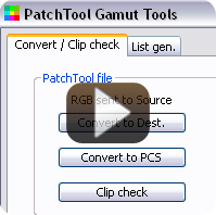
![]() Recently, I have also successfully used the new Gamut Tools module in the PatchTool (PT) application (ver. 2.5 and higher). The input R'G'B' ramp values "readable" by PT can be obtained here. Measured LAB values of the monitor can be downloaded here. And finally, the LAB values obtained through the display profile (large933.icm as in the above example) are here. To see the sequence of steps for converting the R'G'B' ramp values into corresponding LAB values in Gamut Tools, review this short Flash video.
Recently, I have also successfully used the new Gamut Tools module in the PatchTool (PT) application (ver. 2.5 and higher). The input R'G'B' ramp values "readable" by PT can be obtained here. Measured LAB values of the monitor can be downloaded here. And finally, the LAB values obtained through the display profile (large933.icm as in the above example) are here. To see the sequence of steps for converting the R'G'B' ramp values into corresponding LAB values in Gamut Tools, review this short Flash video.
[1B] Another approach is to obtain the linearized RGB values together with optimized values of the [3x3] or [3x4] transfer matrix (eq. VI). While this approach is more accurate, it is at the same time more laborious. A series of R'G'B' input values is run through the transform matrix and obtained predicted tristimulus XYZ values are converted to L*a*b*(D50) values. Determined linearized values do not necessarily have to be identical to those found from the above icc-based technique. The reason is that profiles describe the calibration and if there was any irregularity in the calibration (video LUT) data, the profile would try to correct for it (that is why many more color samples are measured during profiling). Following this approach, we will later evaluate several linearization models and matrices for the display characterization.
1.1. Results of the Display Characterization:
Temporal stability:
Since the backlight fluorescent tubes require certain warm up time in order to reach the stable luminance and chromaticity output (15 - 30 minutes is typically recommended before monitor calibration and profiling), it is reasonable to expect that Eizo LCD monitor will exhibit some warm up characteristics. Thus the very first measurement was to examine the Eizo display's temporal stability on the basis of the luminance and the colorimetric stability of the displayed white color. The first spectrum was measured by the Eye1 Pro spectrophotometer immediately after turning on the display (after being turned off for 15 min). The remaining measurements followed in temporal intervals of 1 minute for the total of 2 hours.
Figure 1 illustrates the percent change in CIE-Y luminance values (cd/m2) from the maximum achieved value of the display white over the 2-hour warm up period. The results are just excellent. The output level increases slightly (0.2 %)
| Figure 1: Percent of luminance (cd/m2) change over a 2-hour warm up period. |
|---|
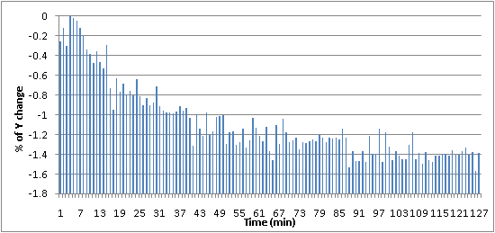 |
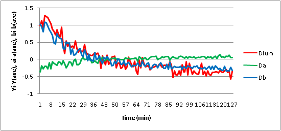
within the first 4 min and then starts to decrease for about 90 min before the full stabilization. the total decrease is however only about 1.4 %, not noticeable at all at output level of 120 cd/m2. In absolute values, the decrease was from 120.0 cd/m2 to 118.5 cd/m2. Figure 2 is more interesting. It illustrates the CIE-Y and CIELAB a*, b* values subtracted from the corresponding average values of the display white over the 2-hour warm up period. There is again a noticeable, although negligible decrease in luminance (~ 1.2 cd/m2) accompanied by changes in the CIELAB color components. While the a* component moves slightly toward the magenta area (+a*), the b* component shows more pronounced drift toward the negative (bluish) values (-b*). Mind you that both drifts are again very small and cannot be registered by the human eye. The consequence, however, is that the white point of the monitor shifts slightly towards the higher CCT. Measurements showed a shift from 6,560 K to 6,680 K.
| Figure 2: Delta of Y and CIELAB a*, b* values over a 2-hour warm up period. |
|---|
 |
Overall, these results suggest that Eizo CG19 monitor has some sort of light stabilization/compensation sensor that quickly corrects for the shifts in brightness, a feature not seen in many LCD monitors. And indeed, Eizo's white paper explains the so called drift correction mechanism for this line of monitors: "... brightness of the backlight stabilizes at the preset value within a few seconds after startup and when it exceeds the preset value the backlight sensor quickly detects the situation and sends a signal to the backlight drive circuit to achieve stable brightness at the preset value".
In conclusion, the temporal stability of this monitor is excellent although small drifts in color and luminance (~ 1-2 %) are detectable by the Eye1 Pro spectrophotometer. For the practical work with images, this is of no consequence when editing or color correcting displayed images. For calibration/profiling purposes, obtained data suggests to wait for about an hour to ensure complete stability of the monitor.
Additivity and color constancy:
The tristimulus values of the red, green, and blue channels at their highest output should add to equal the tristimulus values of the display white. Perfect additivity is rarely achieved for all three channels. In this example, the measured white's tristimulus values (X,Y,Z = 95.59, 100.00, 108.96) were lower than the sum of measured primaries at their highest output (X,Y,Z = 96.50, 100.81, 110.76). However, the average difference of 1.1% indicates excellent additivity.
To assess the channel scalability (proportionality), measured tristimulus values of each ramp were converted to CIE (x,y)-chromaticities and plotted in Figure 3. If each channel has scalable tristimulus values, its ramp chromaticities will plot as a single point (chromaticities are invariant to changes in level). When tristimulus values are not corrected for the black level (flare), scalability is clearly violated (panel A). Chromaticities of each channel "wander off" toward the black point. As a comparison, the chromaticities of each channel after subtracting the black level from the tristimulus XYZ data are shown in the panel B.
| Figure 3: Chromaticities of primary ramps w/o flare correction |
|---|
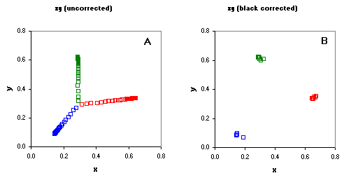 |
For the higher input values the display exhibits acceptable chromaticity constancy, whereas for the measurements in low luminance region, the chromaticity coordinates show noticeable aberrations. It is clearly evident that even after correction for the black-level flare, each channel's chromaticities vary with the luminance. This would suggest that the spectral transmittance of a liquid crystal varies as a function of input voltage. It is important to watch the channel scalability as the successful use of the linear RGB->XYZ and XYZ->RGB transformations depend on it (see eq. XIII and eq. XIV).
[1A] - ICC - using the A2B1 table:
Before going into more complex models, let's take a look at the results that use the CLUT table of the display icc profile. In this particular case, LUT-based profile (large933.icm) was used that has been created in "Argyll" section of these web pages.
Ramps:
We will start with the colorimetric assessment of the RGB ramps. Most of the presented data can be obtained from the Ramps_XYZ.xls spreadsheet (see the "Data processing" above). However, tables and pictures shown in this section come from the code written in Matlab® (send me an e-mail if interested). Table 1 shows the three main parameters used in the display characterization, namely the average CIEDE2000, standard deviation of CIEDE2000 (sigma), and the maximum
| Channel | Ave DE2000 | Sigma DE2000 | Max DE2000 |
|---|---|---|---|
| RGB | 1.15 | 0.76 | 2.99 |
| R | 0.85 | 0.54 | 2.86 |
| G | 0.79 | 0.51 | 2.99 |
| B | 1.80 | 0.73 | 2.78 |
CIEDE2000. These statistical descriptors were calculated for both the three ramps together and for each RGB channel separately. Overall, values are rather high suggesting that this LUT-based icc profile is not the ideal source of "theoretical" L*a*b* values for the RGB ramps. More examples would be needed to come to more conclusive statement. Because CLUT tables are results of a multiparameter optimization with colors being estimated by an interpolation within the table 3-D grid, it would not be completely surprising if icc profiles would perform worse than theoretical models in this comparison. Furthermore, the performance of the LUT tables depend on the "age" of the calibration.
| Figure 4: A2B1 - DE2000 for RGB channels |
|---|
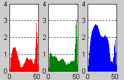 |
More detailed analysis of the same data is shown in Figure 4 . Values on the x-axis correspond to digital counts expressed as R', G', and B' ( in 5-step increments). Value of 0 at the x-axis corresponds to 255 and value of 51 corresponds to R'=G'=B'=0. In other words, the brightest colors are on the left, the darkest tones are on the right. Values on the y-axis are the DE2000 color differences for each channel. From these histograms, it is clear that performance of the blue channel is compromised. Again, the use of A2B1 table of this icc profile results in rather average description of the primary color ramps at the gamut boundary.
![]() Same analysis done in the Patch Tool application can be reviewed in this short Flash video. Required files were created in Gamut Tools excercise above.
Same analysis done in the Patch Tool application can be reviewed in this short Flash video. Required files were created in Gamut Tools excercise above.

Color Patches:
In contrast to the RGB ramps, LUT-based icc profile performs much better in predicting the "theoretical" L*a*b* values of the color patches. Table 2 summarizes the average CIEDE2000, standard deviation of CIEDE2000 (sigma), and the maximum CIEDE2000 of 31 gray steps and 122 color patches, respectively. Since number of color and gray patches
| Color (#) | Ave DE2000 | Sigma DE2000 | Max DE2000 |
|---|---|---|---|
| Gray (31) | 0.30 | 0.18 | 1.02 |
| Colors (122) | 0.31 | 0.23 | 1.27 |
| Figure 5: A2B1 - DE2000 for color patches |
|---|
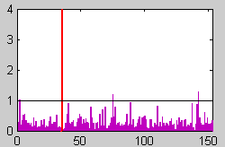 |
differ, direct comparison of the statistical descriptors cannot be made. However, the values are still in ranges where color differences are hardly noticeable. Figure 5 shows distribution of the CIEDE2000 values across the whole range of the color patches.
| Figure 6: A2B1 - DE2000 for color patches |
|---|
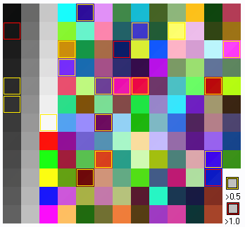 |
Bars left of the red vertical line are the gray steps, bars to the right are the color patches. Black horizontal line indicates the threshold value of 1 for the DE2000 (JND). Inspection of Figure 6 reveals that larger DE2000 values come from the darker patches with some bias toward the blue region. CIEDE2000 differences in the grayscale patches are acceptable with some weaker areas in darks. Patches outlined in yellow have DE2000 > 0.5, patches outlined in red have DE2000 > 1.0.
In summary, this LUT- icc profile provides very reasonable "theoretical" L*a*b* values of the color patches. However, as in the ramp analysis, the weakness in blue areas is still apparent.
Grayscale:
Quality of the grayscale response is very important, especially when working with black and white images. The quality is best judged by a visual inspection of a grayscale image displayed through a color managed application or directly on the calibrated screen. In general, to assess quality of the current calibration, look first at the calculated log-log gamma and the measured white point. The former is directly calculated in the spreadsheet Gray_XYZ.xls, the latter is
| Profile | Ave DE2000 | Sigma DE2000 | Max DE2000 |
|---|---|---|---|
| LUT | 1.27 | 0.58 | 3.37 |
| Shaper/M | 1.34 | 0.39 | 2.53 |
| Figure 7: A2B1 - DE00 for color patches |
|---|
 |
best estimated from the Bruce Lindbloom's CIE Color calculator. In this specific example, measured gamma of the display was 2.20 (2.20 requested). Linear regression was performed on the log-log plot of Yn vs. RGBn. The sum of squares due to error (SSE) was 7.7e-5 and the R2=0.9999. This is an excellent fit confirming the gamma parameter. The CCT of this calibrated state was 6,528 K (6,500 K requested). These are excellent results. However, detailed analysis of the measured and predicted L*a*b* values shows color differences
| Figure 8: LAB (a*,b*) profile of the gray patches |
|---|
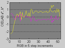 |
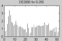
larger than those shown for gray patches in the previous section (Fig. 6). This observation is rather surprising and indicates that there are other sources of color differences between those measurements. Table 3 compares results of two different methods for obtaining the "theoretical" CIELAB data. In one case, the LUT-based profile was used, in the other case, the smaller shaper-matrix profile was used. The LUT-based profile seems to perform slightly better although there are more unevenly distributed areas of the DE2000 (greater sigma value). From the visual inspection, the grayscale gradient (with sRGB profile attached) shown through the large display LUT profile has smoother shadows than when sent through the smaller shape-matrix profile. However, the differences are rather small. Figure 7 shows the distribution of DE2000 values across the whole range of the RGB gray values (from black to white, LUT-based). Performance in the region below RGB=50 (x-value of 10) is clearly suboptimal. Even more detailed analysis (Fig. 8 ) reveals that it is the b* component (yellow-blue) of the LAB system that causes the problem. Negative values of b* in shadows indicate a blue tint (fortunately not visible due to poor sensitivity of human vision at low luminance values). Complete analysis of the L*a*b* values (not shown) indicates that lightness (L*) also causes poor behavior in the shadows.
(top)↑Last update : June , 2009

Eizo CG19 line of LCD displays.
Display gamma estimation applet from Hans Brettel.
For color conversions, spectral measurements, and color space transformations , I prefer the BabelColor Color Translator and Analyzer (CT&A) written and frequently updated by Danny Pascale.
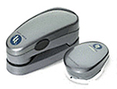
Eye1 Pro spectrophotometer (left) and the Eye1 Display colorimeter (right) .